In previous examples I used both Gaussian plume and puff models for continuous and instantaneous releases, respectively, but what about the in-between cases? It is more commonly the case for a leak from a process vessel to be a prolonged, but finitely long, release.
The guidance is to typically pick one or the other, depending upon the length of the release, or use a more complex model, e.g. the guidance in LeesLees, Loss Prevention, 15/199. is
| \(u \Delta t \lt 2 \sigma_x\) | Use puff model |
| \(2 \sigma_x \lt u \Delta t \lt 5 \sigma_x\) | Neither model entirely appropriate |
| \(u \Delta t \gt 5 \sigma_x\) | Use plume model |
Where u is the wind speed, Δt the duration of the release, and $\sigma_x$ is the downwind dispersion evaluated at \(x = \frac{u \Delta t}{2}\) These criteria drive one to using a plume model in most cases that are not “instantaneous”. Suppose $\sigma_x = \alpha x^\beta$ then the criteria for a puff is $u \Delta t \lt 2 \alpha^{1 \over 1-\beta}$ which, for a class D release with windspeed of 2m/s works out to $\Delta t \lt 5 \times 10^{-16} \mathrm{s}$. The criteria for a plume is $u \Delta t \gt 2 \left( 2.5 \alpha \right)^{1 \over 1-\beta}$ which works out to $\Delta t \gt 5 \times 10^{-11} \mathrm{s}$ for the same situation. So for any release of appreciable duration it will be a plume.
An alternative approach is to evaluate the downwind dispersion at a particular point of interest x1 and use the same criteria. This is much less strict than what Lees gives and is what I will do, it motivates investigating anything other than pure plume models.
One approach in this in-between zone is to try both and pick the most conservative. But that can lead to extremely conservative results. An alternative might be to take a page from more complex models, such as INTPUFF and SCIPUFF, and treat an intermediate release as a series of smaller puff releases.
Motivating example
Suppose a release from a process vessel, say a jet of gas issuing from a hole, we suppose the release is a constant rate of 1kg/s for 5s just for some nice round numbers. The release is at ground level and the ambient conditions are class D with a 2m/s windspeed. We have a point of interest 100m down-wind of the release, this could be an inhabited building or the fence-line.We are also implicitly assuming the release is neutrally buoyant, and so a Gaussian dispersion model would be appropriate.
m  = 1 #kg/s
Δt = 5 #s
h  = 0 #m
u  = 2 #m/s

x₁ = 100  #m
t₁ = x₁/u #s
50.0
The class D dispersion parametersAIChE/CCPS Guidelines for Consequence Analysis, 90. are:
# class D puff dispersion

σx(x) = 0.06*x^0.92
σy(x) = σx(x)
σz(x) = 0.15*x^0.70
The release, at the point of interest, meets neither the criteria for a puff model nor a plume model.
u*Δt < 2*σx(x₁)
false
u*Δt > 5*σx(x₁)
false
So some other kind of model must be used.
Single Gaussian puff
Recall that a single Gaussian puff is the product of 3 Gaussian distributions
\[c \left(x,y,z,t \right) = m \Delta t \cdot g_x(x, t) \cdot g_y(y) \cdot g_z(z)\]with
\[g_x(x,t) = {1 \over \sqrt{2\pi} \sigma_x } \exp \left( -\frac{1}{2} \left( x-u t \over \sigma_x \right)^2 \right)\] \[g_y(y) = {1 \over \sqrt{2\pi} \sigma_y } \exp \left( -\frac{1}{2} \left( y \over \sigma_y \right)^2 \right)\] \[g_z(z) = {1 \over \sqrt{2\pi} \sigma_z } \left[ \exp \left( -\frac{1}{2} \left( z-h \over \sigma_z \right)^2 \right) + \exp \left( -\frac{1}{2} \left( z+h \over \sigma_z \right)^2 \right) \right]\]where, for the sake of clarity, I’ve neglected the fact that the dispersion parameters σ are themselves all functions of t by being functions of the location of the center of the puff.
gx(x, t) = exp((-1/2)*((x-u*t)/σx(u*t))^2)/(√(2π)*σx(u*t))
gy(y, t) = exp((-1/2)*(y/σy(u*t))^2)/(√(2π)*σy(u*t))
gz(z, t) = (exp((-1/2)*((z-h)/σz(u*t))^2)+exp((-1/2)*((z+h)/σz(u*t))^2))/(√(2π)*σz(u*t))
c_pf(x,y,z,t; m, Δt) = m*Δt*gx(x,t)*gy(y,t)*gz(z,t)
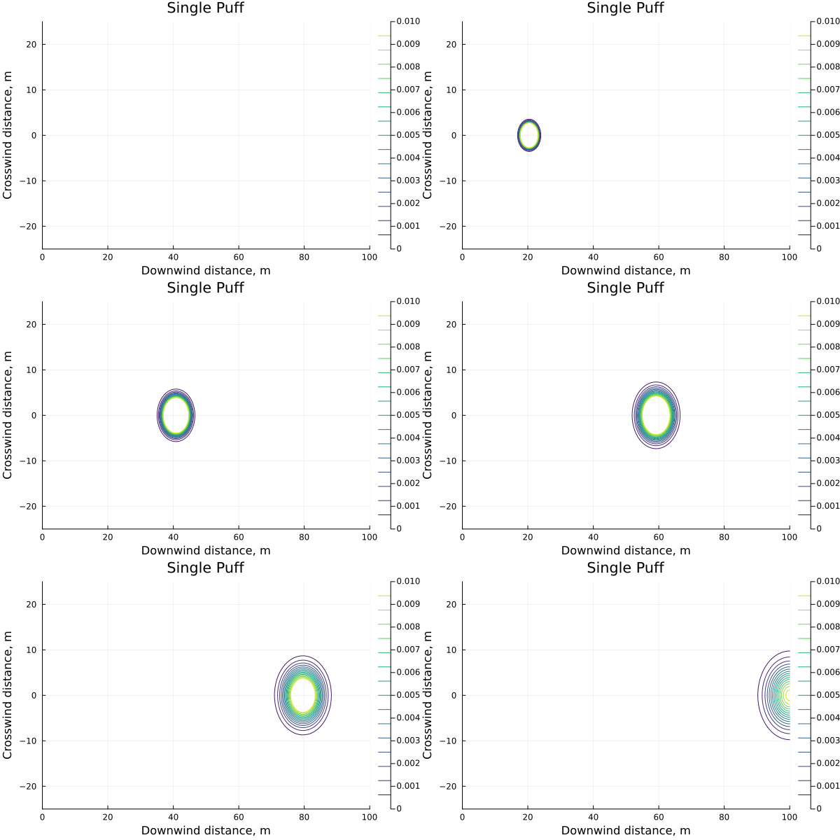
For some context we can plot the puff as a single, instantaneous, release

Multiple puffs
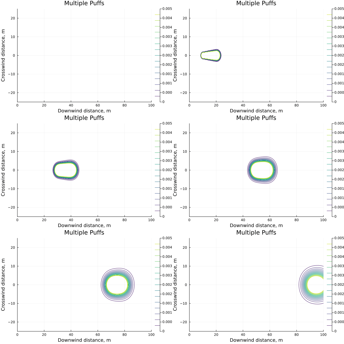
Our first approximation to a release of appreciable duration is to break the release up into n intervals and release a single puff per interval.
\[c(x,y,z,t) = \sum_{i=0}^{n} m \frac{\Delta t}{n} \cdot g_x(x, t-\frac{i}{n}\Delta t) \cdot g_y(y) \cdot g_z(z)\]where we have simply taken the sum of n single puffs, each representing a fraction of the overall release, and emitting them one after the other.
function sum_of_puffs(x,y,z,t; m, Δt, n)
    c = 0
    δt = Δt/n
    for i in 0:1:n
        t′ = t-i*δt
        c′  = t′>0 ? c_pf(x,y,z,t′; m=m, Δt=δt) : 0
        c += isnan(c′) ? 0 : c′
    end
    return c
end
We can plot this for n=5 and we see that, while initially the individual puffs are distinct, they quickly merge into a larger more spread-out cloud.To an extent this is a function of using a class D atmosphere. For a much more stable atmosphere, e.g. class F, the puffs remain quite distinct until a size-able number of them have been released.

If we plot the max-concentration experienced at our point of interest, x=100m, against an increasingly finely-divided release (more puffs, but each puff represents a smaller slice of time) it is clear that they are converging towards a number, and relatively quickly.
This suggests a next step, taking the limit as $n \to \infty$
Integrated puffs
Returning to our model of multiple puffs
\[c(x,y,z,t) = \sum_{i=0}^{n} m \frac{\Delta t}{n} \cdot g_x(x, t-\frac{i}{n}\Delta t) \cdot g_y(y) \cdot g_z(z)\]We can re-arrange this and take the limit as $n \to \infty$
\[c(x,y,z,t) = m\cdot g_y(y) \cdot g_z(z) \cdot \left( \lim_{n \to \infty} \sum_{i=0}^{n} g_x(x, t-\frac{i}{n}\Delta t) \frac{\Delta t}{n} \right) \\ = m\cdot g_y(y) \cdot g_z(z) \cdot \int_{t-\Delta t}^{t} g_x(x, t^{\prime}) dt^{\prime}\]Where we have replaced the limit with the integral.I am assuming the dispersion parameters are constants, though they are not in practice as they are correlated to the downwind distance to the center of any given puff. I am assuming for a small enough release this is approximately constant at least.
This is an integral of a Gaussian, and so we expect the results to be in terms of the error function
\[\mathrm{erf}(x) = \frac{2}{\sqrt{\pi}} \int_0^x \exp \left( -t^2 \right) dt\]For the integral of the x component of the Gaussian puff we have \(\int_{t-\Delta t}^{t} g_x(x, t^{\prime}) dt^{\prime} = \int_{t-\Delta t}^{t} {1 \over \sqrt{2\pi} \sigma_x } \exp \left( -\frac{1}{2} \left( x-u t^{\prime} \over \sigma_x \right)^2 \right) dt^{\prime}\)
making the substitution \(\xi = { {x - u t^{\prime} } \over \sqrt{2} \sigma_x}\)
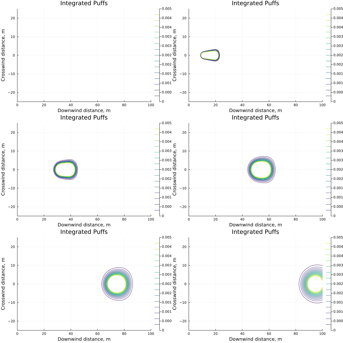
we getThis model and the sum of puffs model both naively include contributions from releases that haven’t happened yet, e.g. at t=1 only the contribution of material released at times t≤1 should be included, but without any correction the other parts of the release would be included causing slight errors in the vicinity of the release point at t<Δt. The solution is simply to take the duration of the release to be the minimum of either the elapsed time (i.e. when the release is still “happening”) or the total release duration.
\[\int_{t-\Delta t}^{t} g_x(x, t^{\prime}) dt^{\prime} = {-1 \over \sqrt{\pi} u} \int_{a}^{b} \exp \left( -\xi^2 \right) d\xi \\ = {-1 \over \sqrt{\pi} u} \left[ \frac{\sqrt{\pi}}{2} \mathrm{erf}(b) - \frac{\sqrt{\pi}}{2} \mathrm{erf}(a) \right] \\ = \frac{1}{2u} \left( \mathrm{erf}(a) - \mathrm{erf}(b) \right)\]where \(a = { {x - u (t-\Delta t)} \over \sqrt{2} \sigma_x }\), \(b = { {x - u t} \over \sqrt{2} \sigma_x }\)
using SpecialFunctions: erf

function ∫gx(x,t,Δt)
    Δt = min(t,Δt)
    a  = (x-u*(t-Δt))/(√2*σx(u*(t-Δt)))
    b  = (x-u*t)/(√2*σx(u*t))
    return erf(b,a)/(2u)
end

intpuff(x,y,z,t; m, Δt) = m*gy(y,x/u)*gz(z,x/u)*∫gx(x,t,Δt)

This release model has some convenient properties: clearly as $\Delta t \to 0$ it becomes a Gaussian puff again, but also as $\Delta t \to \infty$ also limits to the Gaussian plume.This is somewhat hand-wavy but a release of infinite duration is an event that began an infinite amount of time in the past and continues an infinite amount into the future, so the term $\frac{1}{2u} \left( \mathrm{erf}(a) - \mathrm{erf}(b) \right)$ goes in the limit to $\frac{1}{2u} \left( \mathrm{erf}(\infty) - \mathrm{erf}(-\infty) \right) = \frac{1}{u}$ resulting in a concentration profile of $ c \left(x,y,z,t \right) = \frac{m}{u} \cdot g_y(y) \cdot g_z(z) $, which is exactly a plume model.
Complications
I’ve been casually treating the dispersion parameters, $\sigma_x, \sigma_y, \sigma_z$, as being constants that are independent of the model and any transformations on the model. Within the context of taking sums and doing integrals it is reasonable: within a reasonable radius of the center of a given puff they are nearly constant. However, in practice, they depend upon time through their dependence on the location of the puff center and are also functions of the model itself.
The dispersion parameters for a plume model are not the same as for a puff, and so the nice smooth curve connecting the two doesn’t really work. Not if you are strictly taking dispersion parameters as provided in standard references. It is not at all clear how to transition from the one set to the other either, in a smooth manner, to ensure that there is a smooth transition from puff to plume.
That said, multiple puff models use the dispersion parameters for puffs and so using the puff parameters in the integrated puff model at least puts one in good company.
Update: There is a follow-up post that discusses the quality of these approximations in more detail.
For a complete listing of code used to generate data and figures, please see the corresponding julia notebook
References
- AIChE/CCPS. Guidelines for Consequence Analysis of Chemical Releases. New York: American Institute of Chemical Engineers, 1999.
- Lees, Frank P. Loss Prevention in the Process Industries. 2nd ed. Oxford: Butterworth-Heinemann, 1996.


Comments