
Very often, in chemical engineering, the line between problems one can solve one’s self and problems that are solved with a piece of commercial software is when ideal fluid assumptions break down. Relief valve sizing is a typical example: if the fluid is (approximately) an ideal gas then sizing is simple and often done in a spreadsheet. When this isn’t the case, if the compressiblity is <0.8 or >1.1,API 520, 68. then one typically has to turn to some commercial software. Models of real fluids are complicated and extracting the relevant thermodynamic properties from them can be quite tedious when doing it all from scratch.
Clapeyron.jl comes to the rescue here with a wide array of equations of state for real fluids. Combined with julia’s robust ecosystem of libraries for integration and optimization, solving real fluid problems becomes simple. This post walks through how to size a relief device, in gas service, starting from an ideal gas and working through various methods for real gases using equations of state.
Sizing a Pressure Relief Valve
The general idea for sizing a relief valve is to determine the minimum area required such that the mass flow through the valve equals the mass flow required for the governing release case via the relationAPI 520, equation B.5
\[W = K A G\]where $W$ is the required mass flow-rate, $K$ is a capacity correction, $A$ is the theoretical flow area, and $G$ the frictionless) mass flux through the valve. Valves are sized based on the theoretical flow area.
The general process is as follows:
- Determine the governing release rate, $W$
- Determine the capacity correction, $K$
- Calculate the mass flux through the valve, $G$
- Calculate the theoretical flow area $A = \frac{W}{K G}$
- Select the appropriate valve with a flow area $>A$.
Standards, such as API 520, give equations that combine steps 3 and 4 and absorb unit-conversions into the constants, so that the equation is in a more convenient form, but this is what is happening under the hood.
The complications creep in through calculating $G$, it is path-dependent and is a function of the equation of state for the fluid. For gas releases the relief device is typically treated as an isentropic nozzle, the assumption being that the flow-rate through the valve is typically large enough that any heat transfer can be neglected.
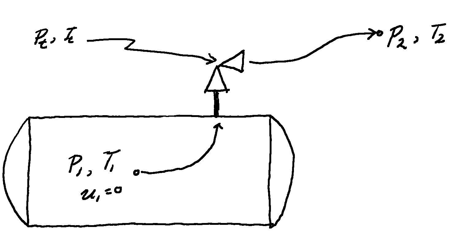
Consider the differential form of the mechanical energy balance, along a streamline from the stagnation point, in the vessel, through the valve and out into the atmosphere, assuming no elevation change and no friction
\[dP + \rho u du = 0\] \[u du = -\frac{dP}{\rho} = - vdP\]Integrating from the stagnation point to the throat of the nozzle gives
\[\frac{1}{2} u_t^2 = - \int_{P_1}^{P_t} v dP\]Where the velocity at the stagnation point, $u_1=0$. Putting this in terms of the mass flux $u = v G$
\[\frac{1}{2} v_t^2 G_t^2 = - \int_{P_1}^{P_t} v dP\] \[G_t = \frac{1}{v_t} \sqrt{-2 \int_{P_1}^{P_t} v dP} = \rho_t \sqrt{2 \int_{P_t}^{P_1} v dP}\]This integral cannot be solved directly at this point as the conditions at the throat of the nozzle are not known. Solving this requires simultaneously solving for the nozzle conditions, $P_t, T_t$.
If we specify that the streamline follows an isentropic path, then we can construct a constrained maximization problem: the nozzle conditions are the $P_t$ and $T_t$ which maximizes $G_t$ where the integration is taken along an isentropic path.
Choked Flow
In the case where flow is choked, i.e. the flow in the nozzle reaches sonic velocity, the maximum $G_t$ occurs at the sonic velocity with a pressure $P_t > P_2$. This can allow for the direct calculation of the mass flux as $G_t = \rho_t c_t$, where $c_t$ is the sonic velocity at the throat. No integration required.
A Motivating Example
Consider the release of ethane from a vessel at 200 bar and 400 K, for the sake of simplicity assume the release is directly into the atmosphere at 1 bar and 288.15 K (15°C) (the flow is going to be choked, so this doesn’t actually matter).
using Unitful
begin
# the vessel properties
    P₁ = 200u"bar"
    T₁ = 400u"K"

# the ambient properties
    P₂ = 1u"bar"
    T₂ = 288.15u"K"
end
We can use Clapeyron.jl to initialize a few example equations of state for ethane. In this case I’m going to use an ideal gas model (ReidIdeal is an ideal gas model that also includes correlations for the ideal gas heat capacity), a cubic equation of state (volume translated Peng Robinson), and an empirical Helmholtz model (GERG-2008).
using Clapeyron
begin
# assorted equations of state for ethane
    ig_ethane = ReidIdeal(["ethane"])
    vtpr_ethane = VTPR(["ethane"]; idealmodel = ReidIdeal)
    gerg_ethane = GERG2008(["ethane"])
end
# this is a hack, ideal models in Clapeyron do not return a
# molar weight and so cannot return a mass density
Clapeyron.mw(model::IdealModel) = Clapeyron.mw(vtpr_ethane)
At system conditions ethane is a super critical fluid, with the temperature and pressure above the critical point, which can be modelled as a dense gas.
The Ideal Gas Case
Considering the choked flow case, we know that $G_t = \frac{c_t}{v_t}$ and, for an ideal gas, the sonic velocity is given byTilton, “Fluid and Particle Dynamics,” equation 6-113.
\[c = \sqrt{ {k R T} \over M} = \sqrt{k P v}\]Combining these we have
\[G_t = \frac{c_t}{v_t} = { \sqrt{ k P_t v_t } \over v_t } = \sqrt{ k P_t \over v_t }\]It can be shown that, along an isentropic path defined by $P v^k = \mathrm{const}$, the critical pressure ratio isTilton, “Fluid and Particle Dynamics,” equation 6-119.
\[{P_t \over P_1} = { P_{chk} \over P_1 } = \left(2 \over {k+1} \right)^{k \over {k-1} }\]Which allows us to write
\[P_t = P_1 {P_t \over P_1} = P_1 \left(2 \over {k+1} \right)^{k \over {k-1} }\]and (using $P_1 v_1^k = P_t v_t^k$)
\[v_t = v_1 \left(P_1 \over P_t \right)^{1 \over k} = v_1 \left(2 \over {k+1} \right)^{-1 \over {k-1} }\]Substituting back into the equation for $G_t$API 520, equation B.21
\[G_t = \sqrt{ k \frac{P_1}{v_1} \left(2 \over {k+1} \right)^{k+1 \over {k-1} } }\]or, to put it in terms of density
\[G_t = \sqrt{ k P_1 \rho_1 \left(2 \over {k+1} \right)^{k+1 \over {k-1} } }\]where $k$, the isentropic expansion factor for an ideal gas, is the ratio of heat capacities
\[k = { c_{p,ig} \over c_{v,ig} }\]This is the basis of API 520 Part 1 equation 9 where the following substitutions is made:
\[\rho = { {P M} \over {Z R T} }\]and the constant $R$ and some unit conversions are rolled up into the constant 0.03948 in the expression for $C$
\[R = 8.314 { {\mathrm{m^3} \cdot \mathrm{Pa} } \over {\mathrm{mol} \cdot \mathrm{K} } } = 8,314 { {\mathrm{m^3} \cdot \mathrm{Pa} } \over {\mathrm{kmol} \cdot \mathrm{K} } } = 8,314 { {\mathrm{kg} \cdot \mathrm{m^2} } \over { \mathrm{kmol} \cdot \mathrm{s^2} \cdot \mathrm{K} } }\] \[{1 \over \sqrt{8,314} } \left[ { \sqrt{ \mathrm{kmol} \cdot \mathrm{K} } \cdot \mathrm{s} } \over { \sqrt{\mathrm{kg} } \cdot \mathrm{m} } \right] \times 3600 \left[ \mathrm{s} \over \mathrm{h} \right] \times 10^{-6} \left[ \mathrm{m^2} \over \mathrm{mm^2} \right] \times 10^3 \left[ \mathrm{Pa} \over \mathrm{kPa} \right] \\= 0.03948 \left[ \sqrt{\mathrm{kmol} \cdot \mathrm{kg} \cdot \mathrm{K} } \over { \mathrm{h} \cdot \mathrm{mm^2} \cdot \mathrm{kPa} } \right]\]We can use Clapeyron.jl to calculate $k$ at any given temperature, using correlations for the ideal gas heat capacity.
function isentropic_expansion_factor(model::IdealModel, P, T; z=[1.0])
    cₚ_ig = isobaric_heat_capacity(model, P, T; phase=:vapor)
    cᵥ_ig = isochoric_heat_capacity(model, P, T; phase=:vapor)
    return cₚ_ig/cᵥ_ig
end
From which we calculate k= 1.146.
We can check our work by comparing with the tabulated values. At 15°C and 1 atm we calculate k= 1.193 which is the same as the tabulated value of 1.19 (given at 15°C and 1 atm).API 520, 70.
function mass_flux_choked(model, P, T; z=[1.0])
    k = isentropic_expansion_factor(model, P, T; z=z)
    ρ = mass_density(model, P, T, z; phase=:vapor)
    Gₜ² = k*P*ρ*(2/(k+1))^((k+1)/(k-1))
    return √(Gₜ²)
end
The theoretical mass flux for the ideal gas is then 38359 kg m^-2 s^-1
The ideal gas model, when the flow is choked, calculates the mass flux directly without needing to calculate the actual conditions at the nozzle. These can be calculated easily as well.Tilton, “Fluid and Particle Dynamics,” equations 6-119 and 6-120.
nozzle_pressure_ideal(P, T, k) = P*(2/(k+1))^(k/(k-1))
nozzle_temperature_ideal(P, T, k) = T*(2/(k+1))
The pressure at the nozzle is 115 bar the temperature at the nozzle is 373 K, which is above the critical point. The fluid supercritical and choked when leaving the PSV.
The Isentropic Expansion Factor
At the vessel conditions, the VTPR model of ethane gives a compressibility factor of 0.672 (GERG-2008 model gives a similar value of 0.69), well below 0.8 and therefore outside the range where the ideal gas model is expected to work well.
An alternative method is to calculate what the effective isentropic expansion factor would be, for the real gas, assuming that the real fluid obeys
\[P_1 v_1^n = P_t v_t^n\]where $n$ is a constant.
The derivation of $n$ follows from the definition of the speed of sound in a gasTilton, “Fluid and Particle Dynamics,” 6-22; Gmehling et al., Chemical Thermodynamics, 113
\[c = \sqrt{ \left( {\partial P} \over {\partial \rho} \right)_S} =\sqrt{ -v^2 \left( {\partial P} \over {\partial v} \right)_S}\]The constant entropy partial derivative can be re-written to eliminate entropyGmehling et al., Chemical Thermodynamics, 660
\[\left( {\partial P} \over {\partial v} \right)_S = { { \left( {\partial S} \over {\partial T} \right)_P \left( {\partial P} \over {\partial T} \right)_v } \over { \left( {\partial S} \over {\partial T} \right)_v \left( {\partial v} \over {\partial T} \right)_P } }\]Using the relationsGmehling et al., Chemical Thermodynamics, equations C.21 and C.8 (respectively)
\[c_p = T \left( {\partial S} \over {\partial T} \right)_P\]and
\[c_v = T \left( {\partial S} \over {\partial T} \right)_V\]we get
\[\left( {\partial P} \over {\partial v} \right)_S = {c_p \over c_v} \left( {\partial P} \over {\partial v} \right)_T\]and the sonic velocity is then
\[c = \sqrt{ -v^2 {c_p \over c_v} \left( {\partial P} \over {\partial v} \right)_T }\]equating this to the ideal gas case, $c = \sqrt{n P v}$, and solving for $n$ givesAPI 520, equation B.13
\[n = -\frac{v}{P} {c_p \over c_v} \left( {\partial P} \over {\partial v} \right)_T\]where $n$ has been used to distinguish it from $k$ (the ideal gas case). This is the version of $n$ presented in most references, such as API 520. The derivation, however, hints at a useful shortcut to calculating $n$ that does not require digging into the internals of Clapeyron.jl to retrieve partial derivatives:
The remainder of the calculations are identical as the ideal gas case, simply substituting $n$ wherever $k$ appears. Unfortunately $n$ is not actually constant and depends on the temperature and pressure, which are not actually known in the nozzle, so the temperature and pressure at the stagnation point are often used instead.
function isentropic_expansion_factor(model, P, T; z=[1.0])
    ρ = mass_density(model, P, T, z)
    c = speed_of_sound(model, P, T, z)
    n = ρ*c^2/P
    return n
end
Using effective isentropic expansion factors from the VTPR equation of state, the theoretical mass flux is 57811 kg m^-2 s^-1 ( 59321 kg m^-2 s^-1 from GERG-2008 ). This is quite a bit larger than the ideal case, indicating that the ideal gas law leads to a significantly over-sized PRV, 51.0% larger.

The isentropic expansion factor method works best when $n$ is approximately constant over the isentropic path. As the above figure shows, this breaks down in ethane for pressures greater than ~100 bar. It also shows that the different equations of state start to diverge greatly further into the supercritical regime.
Solving the Choked Flow Energy Balance
Another approach, and one I have seen more often in older references, is to perform an energy balance over the isentropic path and, assuming the flow is choked, solve for sonic velocity in the nozzle.Crowl et al, “Process Safety,” 23-55; Gmehling et al., Chemical Thermodynamics, 603. Consider an energy balance starting at the stagnation point, (1), and following an isentropic path to immediately after the throat of the nozzle (t).
\[h_1 = h_t + \frac{1}{2} c_t^2\]Where $c_t$ is the speed of sound at the nozzle, a function of $P_t$ and $T_t$. The procedure is then to solve the system of equations given by the energy balance and the entropy balance, $s_1 = s_t$, for $P_t$ and $T_t$, then the theoretical mass flux is given by
\[G_t = \rho_t c_t\]There are a few ways this could be done, a straight-forward way is to divide the problem into two:
- Define the isentropic path, i.e. find the isentropic temperature for a given pressure P
- Use the energy balance to solve for the pressure, following the isentropic path.
A more direct way is to solve for $P_t$ and $T_t$ simultaneously. This is what I do next, using NonlinearSolve.jl
# Clapeyron does not expose this by default
molecular_weight(model,z) = Clapeyron.molecular_weight(model,z)
function nozzle_balance(y, prms)
    P, T = y

    # stagnation point
    s₁ = prms.entropy
    h₁ = prms.enthalpy

    # at throat conditions
    s₂ = entropy(prms.model, P, T, prms.z)
    h₂ = enthalpy(prms.model, P, T, prms.z)/prms.Mw
    c² = speed_of_sound(prms.model, P, T, prms.z)^2

    return [ s₁ - s₂
             h₁ - h₂ - 0.5*c² ]
end
function mass_flux_choked_energy_balance(model, P, T; z=[1.0])
    # calculate the entropy and specific enthalpy at
    # initial conditions
    Mw = molecular_weight(model, z)
    s₁ = entropy(model, P, T)
    h₁ = enthalpy(model, P, T)/Mw

    # solve the choked flow energy balance for
    # an isentropic nozzle
    params = (model=model, entropy=s₁, enthalpy=h₁, z=z, Mw=Mw)
    y₀ = [P; T]
    prob = NonlinearProblem(nozzle_balance, y₀, params)
    sol = solve(prob, NewtonRaphson())
    Pₜ, Tₜ = sol.u

    # velocity is the sonic velocity at nozzle conditions
    ρₜ = mass_density(model, Pₜ, Tₜ, z)
    cₜ = speed_of_sound(model, Pₜ, Tₜ, z)

    return ρₜ*cₜ
end
function mass_flux_choked_energy_balance(model, P::Quantity, T::Quantity; z=[1.0])
    P = ustrip(u"Pa", P)
    T = ustrip(u"K", T)
    return mass_flux_choked_energy_balance(model, P, T; z=z)*1u"kg*m^-2*s^-1"
end
Solving the choked flow energy balance, using VTPR equation of state, the theoretical mass flux is 54629 kg m^-2 s^-1 ( 54353 kg m^-2 s^-1 from GERG-2008 ). This is also quite a bit larger than the ideal case, 42.0% larger. Though the values for the two equations of state are closer, indicating that this method is less sensitive to model choice.

In this case the ideal gas method and the isentropic expansion factor method bracket the more exact method of solving the energy balance directly.
As it is written, this method would need to be modified to allow for non-choked flow. This is done by eliminating the assumption $u_t = c_t$ and instead finding the conditions which maximize $G_t$ (subject to the constraints of the entropy balance and the enthalpy balance). This will arrive at the same solution, in the case of choked flow, but with a little more effort.
Direct Integration
Direct integration is the method most commonly recommended today, as it is entirely general. It can be used to solve all flow conditions from liquids to gases as well as two-phase mixtures. As a reminder, this method constitutes finding the $P_t$ and $T_t$ that maximize the mass flux given by
\[G_t = \rho_t \sqrt{2 \int_{P_t}^{P_1} v dP}\]First introduce the change of variables $\Delta P = P_1 - P$ such that the integration is from $0$ to $P_1 - P_2$.
\[\int_{P_2}^{P_1} v dP = - \int_{0}^{\Delta P} v\left( P_1 - \Delta P \right)_{s = s_1} d\left(\Delta P \right)\]This allows us to write the corresponding differential equation
\[{ {d} \over {d \left(\Delta P \right)} } I = v\left(P₁ - ΔP\right)\]subject to the constraint
\[s(P_1 - \Delta P, T) = s(P_1, T_1)\]Which can be implemented as a differential algebraic equation using DifferentialEquations.jl
using DifferentialEquations
function rhs(u, params, ΔP)
    ∫vdP, T = u
    model, P₁, s₁, z, Mw = params
    P = P₁ - ΔP
    return [ volume(model, P, T, z)/Mw
             s₁ - entropy(model, P, T) ]
end
But we want to stop the integration when ${ {\partial G} \over {\partial \left( \Delta P \right) } } = 0$ or, equivalently, when the velocity is sonic. We can show that these are the same by finding the stationary points of $G^2$
\[{ {\partial G^2} \over {\partial \left( \Delta P \right) } } = { {\partial } \over {\partial \left( \Delta P \right) } } \left( 2 \rho_t^2 \int_0^{\Delta P_t} v d \left( \Delta P \right) \right) = 0\]by applying the chain rule and cancelling $\rho$ we get
\[2 \left( {\partial \rho} \over { \partial P } \right)_S \int_0^{\Delta P_t} v d \left( \Delta P \right) - 1 = 0\]recalling the definition of the speed of sound (above)
\[\left( {\partial \rho} \over { \partial P } \right)_S = \frac{1}{c^2}\]we have
\[2 \int_0^{\Delta P_t} v d \left( \Delta P \right) - c^2 = 0\]which is simply restating $u_t = c_t$.
function ∂G²_callback(u, ΔP, integrator)
	∫vdP, Tₜ = u
	model, P₁, s₁, z, Mw = integrator.p
	Pₜ = P₁ - ΔP
	c = speed_of_sound(model, Pₜ, Tₜ, z)
	return 2∫vdP - c^2
end
function mass_flux_direct_integration(model, P₁, T₁, P₂;
                                      z=[1.0], solver=Rodas5P())
    s₁ = entropy(model, P₁, T₁, z)
    Mw = molecular_weight(model, z)

    # defining the ODEFunction
    M = [ 1 0
          0 0 ]
    f = ODEFunction(rhs, mass_matrix = M)

    # defining the ODEProblem
    u0 = [0.0; T₁]
    params = (model, P₁, s₁, z, Mw)
    ΔP_span = (0.0, P₁ - P₂)
    prob = ODEProblem(f, u0, ΔP_span, params)
    cb = ContinuousCallback(∂G²_callback, terminate!)

    # solving the DAE
    sol = solve(prob, solver, callback=cb)

    # unpacking the solution
    ΔPₜ = sol.t[end]
    ∫vdP, Tₜ = sol.u[end]
    ρₜ = mass_density(model, P₁-ΔPₜ, Tₜ, z)
    G = ρₜ*√(2*∫vdP)
end
function mass_flux_direct_integration(model, P₁::Quantity, T₁::Quantity,
                          P₂::Quantity; z=[1.0])
    P_1 = ustrip(u"Pa", P₁)
    P_2 = ustrip(u"Pa", P₂)
    T_1 = ustrip(u"K", T₁)
    return mass_flux_direct_integration(model, P_1, T_1, P_2; z=z)*1u"kg*m^-2*s^-1"
end
Direct integration of the VTPR equation of state gives a theoretical mass flux of 54629 kg m^-2 s^-1 ( 54353 kg m^-2 s^-1 from GERG-2008 ). Which is exactly the same as from solving the choked flow energy balance, as expected.

Writing this as a differential algebraic equation was largely necessary because Clapeyron.jl does not expose any routines to calculate the volume as a function of pressure and entropy. Some libraries like CoolProps do, in which case the code could be simplified to be a one dimensional ode.
This method could be extended to include liquid and two-phase flows however, as it is currently implemented, it only handles gases. Unlike the energy balance method, though, the flow does not have to be choked. If the flow is not choked, the maximum will occur once the nozzle pressure reaches $P_2$. This result will simply pop out without any extra effort.
Comparing the Results
For the sake of completeness, there are two other methods that should be looked at, which are really special cases:
- the ideal gas case, but using the real compressibility, $Z$, at stagnation conditions, this is the API 520 standard approach for gases
- using the isentropic expansion factor, n factor, method but calculating n at the average of the stagnation and nozzle conditions
These two approaches do better than the basic methods I presented, but I don’t think they add enough value on their own. Given a model of the gas which can generate the compressibility, using either the energy balance method or the direct integration method produces superior results than correcting the ideal gas case. Once a viable equation of state is in hand, the simplifications are not saving any actual engineer doing their job time, they are saving fractions of a second of compute time.
I think the choice between the first law energy balance and the direct integration technique is more a matter of taste, at least in the case of choked flow. The direct integration method is in the relevant engineering codes/standards, and that is a strong justification for using it.

In this case the choice of equation of state did not matter strongly, just for fun I have included a few other common cubic equations of state, they all perform reasonably. However this example is for a single compound that is not strongly associating, it is the type of example where cubic equations of state should work well. The choice of equation of state will be far more important with mixtures and strongly associating substances.
Final Thoughts
I have long been an advocate for engineering to move out of using spreadsheets for everything and to use scripting languages and notebooks like Jupyter and Pluto far more. There are large classes of problems that are easy to solve with code and hard to solve with a spreadsheet. I think almost any calculation using equations of state fit into that category. We end up beholden to commercial software suppliers for calculations that, in my view, engineers should be doing themselves.
Presumably you could do the calculations I laid out above in Excel, at enormous effort, and making liberal use of the solver. Julia, however, has a robust ecosystem for doing all the complicated math, it only needed to be connected up. What remains, for the engineer, is assessing the physical system and picking the appropriate methods and thermodynamic models.
For a complete listing of code used to generate data and figures, please see the corresponding pluto notebook
References
- API Standard 520, Sizing, Selection, and Installation of Pressure-relieving Devices, Part I - Sizing and Selection. 10th ed. Washington, DC: American Petroleum Institute, 2020.
- Center for Chemical Process Safety. Guidelines for Pressure Relief and Effluent Handling Systems. 2nd ed. Hoboken, NJ: John Wiley & Sons, 2017.
- Crowl, Daniel A., Lawrence G. Britton, Walter L. Frank, Stanley Grossel, Dennis Hendershot, W. G. High, Robert W. Johnson et al. "Process Safety." in Green, Perry’s Chemical Engineers’ Handbook.
- Green, Don W., ed. Perry’s Chemical Engineers’ Handbook. 8th ed. New York: McGraw Hill, 2008.
- Gmehling, Jürgen, Bärbel Kolbe, Michael Kleiber, and Jürgen Rary. Chemical Thermodynamics for Process Simulation. Weinheim, DE: Wiley-VCH Verlag & Co., 2012
- Tilton, James N. "Fluid and Particle Dynamics." in Green, Perry’s Chemical Engineers’ Handbook.
Comments