
It has been a beautiful spring in Edmonton and the trees are tentatively flowering and throwing pollen to the wind. Watching the trees come back from their barren winter state left me wondering about the wind dispersal of pollen. Pollen grains must be small enough to travel quite a distance to encounter any other trees to pollinate, but they do settle out eventually. So, how far do they actually go? I’ve been wanting to play around with the mapping tools in the julia ecosystem, and this question gave me an opportunity to make some maps exploring pollen dispersal in my neighbourhood.
I live in an older core neighbourhood in Edmonton, which has a beautiful canopy of boulevard trees. Primarily elm, but also ash, maple, and oak. The legacy of people like Gladys Reeves and the Edmonton Tree Planting Committee who, starting in 1923, defended our city green spaces and built up our urban forest. A legacy we still fight for over a century later.
In particular I’m going to be looking at American Elm, the most common boulevard tree in my neighbourhood, and I’ll restrict myself to just here (not the whole city).
Some Notes on Unitful
For a lot of problems, I find it easier to work with Unitful.jl. It enforces unit consistency and inconsistent units in an answer is a good indication that I have made a math mistake somewhere. However there are two questions that I need to answer before getting too deep into things:
- What units am I using for pollen dispersal?
- How will I be handling all the correlations?
I could calculate the pollen concentration on a mass basis, but that seems kind of weird to me. I think the logical unit is in terms of individual pollen grains. That is not a unit that Unitful.jl is aware of and so I need to define first what a pollen grain is. It is a unit of “number”, like a mole, and in fact there are 6.022×10²³ grains in a mole of pollen.
using Unitful
begin

@unit grains "grains" Grains (1/6.02214076e23)*u"mol" true;
Unitful.register(@__MODULE__);

end
Correlations can be annoying with Unitful.jl since the various constants in a correlation are not usually given with units and figuring them all out so that units remain consistent is kind of tedious. The easiest workaround is to use a macro to strip the units off the input to a correlation function and then stick the correct units back on the output.
macro ucorrel(f::Symbol, in_unit::Expr, out_unit::Expr)
   quote
       function $(esc(f))(x::Quantity)::Quantity
           x = ustrip($in_unit, x)
           res = $(esc(f))(x)
           return res*$out_unit
       end
   end
end;
Building a Model of Pollen Dispersion
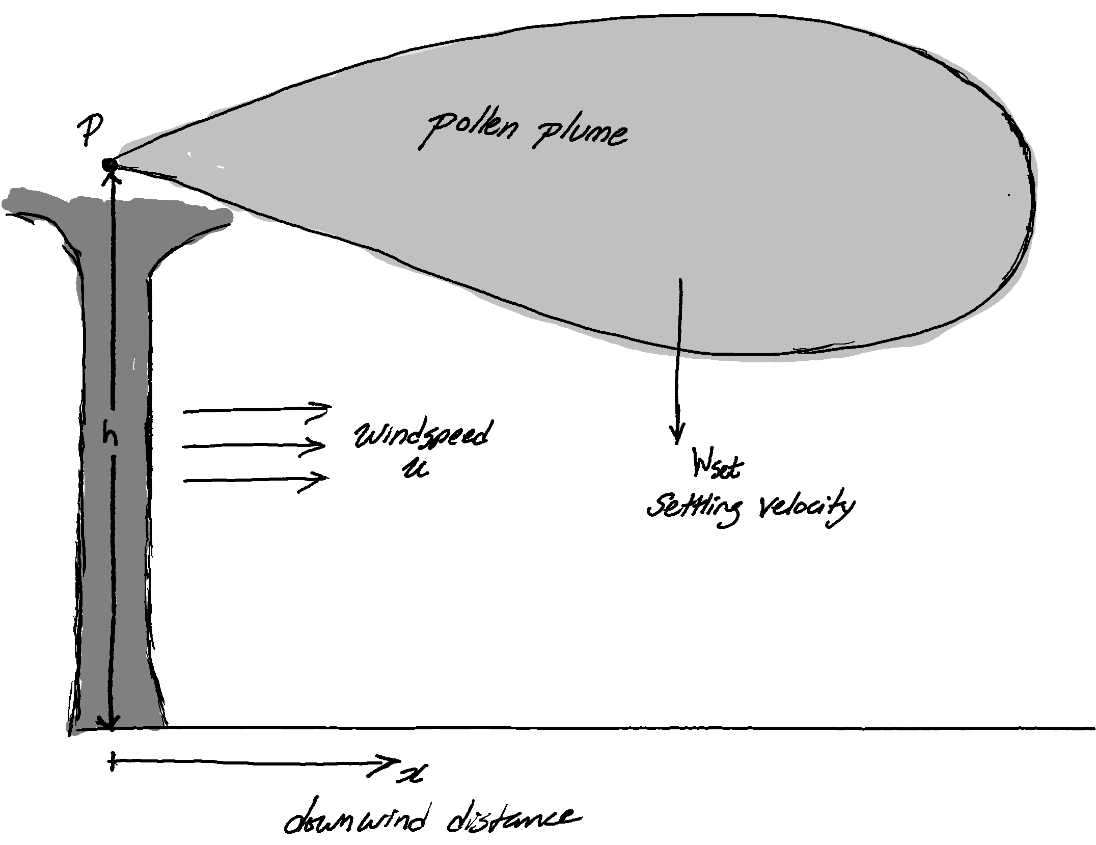
For an initial sketch I’m going to consider a single tree as an elevated point source producing pollen at a constant rate P and with the wind carrying the pollen away with a constant wind speed u. Individual pollen grains settle out of the plume as they are carried downwind with velocity $W_{set}$. The coordinate system is centred at the base of the tree with an x-axis parallel to the wind.
A Model Elm Tree
There are a few things I will need to know about each elm tree in the neighbourhood:
- The height at which pollen is released
- The rate at which pollen is released
Neither of these are typically measured and available in data sets for urban forests. I will need to use correlations – what foresters call allometric equations. These correlate physical parameters of trees to something easier to measure, such as the diameter at breast height or DBH.
To build an example elm tree, suppose it has a DBH of 88 cm
# Model Elm tree
DBH = 88u"cm" |> u"m"
The crown height for an American Elm is correlated to DBH by the following equationMcPherson, van Doorn, and Peper, Urban Tree Database for urban trees in the North climate zone
# McPherson, van Doorn, and Peper, *Urban Tree Database*
# Ulmus Americana, North climate zone
crown_height(DBH) = 0.44998 + 0.55096*DBH - 0.00666*DBH^2 + 3e-5*DBH^3
@ucorrel crown_height u"cm" u"m"
I am going to assume this is the height at which pollen is released, that’s not particularly accurate but it is a start. A better value would be the “centre of mass” for pollen in the crown of an Elm tree, but that isn’t readily available.
For the example tree, this predicts a height of 17.8 m which, just standing around and looking at the trees on my street seems plausible. The example elm tree should be taller than a 5 story building, and there is an elm tree at the end of my block that is about that in both diameter and height.
The total amount of pollen in a given elm tree is given by the following equationKatz, Morris, and Batterman, “Pollen Production,” Table 2 where B is the tree basal area. The total pollen is based on counts of pollen per anther and an estimate of the total number of anthers per tree for urban elm trees in Ann Arbor, Michigan. Maybe not perfectly comparable to Edmonton, but it’s good enough for this exploratory work.
# Ulmus Americana total pollen per tree
# Katz, Morris, and Batterman, "Pollen Production," Table 2
function total_pollen(DBH)
    B = π/4*DBH^2
    return exp(5.86*B + 23.11)
end
@ucorrel total_pollen u"m" u"grains"
This gives a total pollen content of 384,082,918,235 grains for the model elm tree, which sounds like a lot.
Elm trees release their pollen, in Edmonton, somewhere from the end of April to mid May and it usually lasts 1-2 weeks. As a very rough model I’m going to assume each tree releases its pollen at a constant rate over a 2 week period, and that the periods over which each of the trees are releasing overlap.
Δt = 14u"d" |> u"s"
pollen_rate(DBH) = total_pollen(DBH)/Δt
For the example tree, this gives a pollen release rate of 317,529 grains s^-1.
Pollen Settling
Elm pollen is relatively large and will settle out of the air. To account for this I am going to assume the pollen settles with a velocity equal to the terminal velocity given by Stokes’ Law, where each individual pollen grain is a solid sphere.

begin

# Ulmus Americana pollen
# Brush and Brush, "Transport of Pollen," Tables 3 and 12.
d  = 31u"μm" |> u"m"
SG = 1.1
ρ  = SG*1000u"kg/m^3"

end;
begin

g  = 9.80665u"m/s^2" # standard gravity
ρₐ = 1.225u"kg/m^3"  # density of dry air (15°C, 1atm)
μₐ = 17.89e-6u"Pa*s" |> u"kg/m/s" # viscosity of dry air (15°C, 1atm)

end;
# Stokes Law
vₜ = ((ρ - ρₐ)*g*d^2)/(18*μₐ)
This gives a settling velocity for a grain of American Elm pollen in air of 3.22 cm s^-1
Atmospheric Dispersion
We might naively consider the pollen being launched out of the tree like little cannon balls, with a velocity in the x-direction equal to the wind speed and the velocity in the z-direction equal to the terminal velocity of pollen. Assuming a wind speed of 2 m s^-1, then a pollen grain from our example tree would travel 1107 m before hitting the ground. That’s pretty far and also kind of unrealistic. It ignores all the turbulent mixing in the air column which will both loft it to much greater heights and, at times, push it towards the ground.
The turbulent mixing in the air is captured using the dispersion parameters $\sigma_y$ and $\sigma_z$ which are functions of the downwind distance. This gives an average view, averaged over all of the pollen grains. In this case I will be using the Briggs’ correlations for Urban terrain.Briggs, Diffusion Estimation for Small Emissions, 38; Griffiths, “Errors in the Use of the Briggs Parameterization.” I am also assuming class D atmospheric stability.
# wind speed, assumed
u = 2u"m/s"
σ_y(x) = 0.16x/√(1+0.0004x)
@ucorrel σ_y u"m" u"m"
σ_z(x) = 0.14x/√(1+0.0003x)
@ucorrel σ_z u"m" u"m"
The Ermak Equation
I will be using the Ermak equationErmak, “An Analytical Model” to model the dispersion of pollen, which results in a Gaussian-like dispersion but with the pollutant falling out and collecting on the ground. The Ermak equation is the solution to the advection diffusion equation with a constant settling velocity $W_{set}$ and deposition velocity $W_{dep}$
\[\frac{\partial c}{\partial r} - \frac{W_{set}}{K} \frac{\partial c}{\partial z} = \frac{\partial^2 c}{\partial y^2} + \frac{\partial^2 c}{\partial z^2}\]with boundary condition at the ground
\[\left( K \frac{\partial c}{\partial z} + W_{set} c \right)_{z=0} = W_{dep} c|_{z=0}\]where K is the eddy diffusivity and r is defined as
\[r = \frac{1}{u} \int_0^x K dx^{\prime}\]and the other boundary conditions are as for the conventional Gaussian dispersion (e.g. constant mass emissions, m, at a point h above the origin, etc.). This can be solved and put in terms of $\sigma_y$ and $\sigma_z$ as, by definition, $\sigma^2 = 2 r$
\[c = \frac{m}{2\pi u \sigma_y \sigma_z} \exp\left( - \frac{y^2}{2 \sigma_y^2} \right) \exp\left( { - {W_{set} (z-h)} \over {2K_z} } - { {W_{set}^2 \sigma_z^2} \over {8K_z^2} } \right)\] \[\times \left( \exp \left( - \left(z-h\right)^2 \over {2\sigma_z^2} \right) + \exp \left( - \left(z+h\right)^2 \over {2\sigma_z^2} \right) \right.\] \[\left. - { {\sqrt{2\pi} W_o \sigma_z} \over K_z} \exp\left( { - {W_o (z+h)} \over {K_z} } - { {W_o^2 \sigma_z^2} \over {2K_z^2} } \right) \mathrm{erfc} \left( { {W_o \sigma_z} \over {\sqrt{2}K_z} } + { {z + h} \over {\sqrt{2}\sigma_z} } \right) \right)\]where $W_o = W_{dep} - \frac{1}{2}W_{set}$. In practice, relationships for $\sigma$s are much easier to find than Ks and the following is used to recover $K_z$
\[K_z = \frac{1}{2} u \frac{d \sigma_z^2}{dx}\]This follows from the definition of $\sigma_z$ (and r). In this case I am going to generate the $K_z$ using automatic differentiation with ForwardDiff.jl.
using ForwardDiff: derivative
∂ₓσ_z²(x) = 2*σ_z(x)*derivative(σ_z, x)
@ucorrel ∂ₓσ_z² u"m" u"m"
K_z(x; u) = (1/2)*u*∂ₓσ_z²(x)
Models like this, with a point source emitting mass, have nonphysical results in the vicinity of the emission source. The concentration rises sharply and there is a singularity at the source itself. There are many ways of dealing with this, but the easiest is to define a maximum concentration, usually given from a mass balance, and cut off the dispersion model at that. I don’t have any specific upper bound, so I picked a large number simply to prevent the propagation of Inf or other errors.
This is only a problem very close to the source, and I am more interested in concentrations far from the tree, so this is not a concern. A better model would calculate a “virtual origin” for the tree such that the pollen concentration in the crown of the tree was more realistic.
max_pollen = 1e6grains/1u"m^3"
using SpecialFunctions: erfc
function ermak(x, y, z; u=u, h=crown_height(DBH), P=pollen_rate(DBH),
                        W_set=vₜ, W_dep=vₜ, p_max=max_pollen)

    if x<zero(x) || z<zero(z)
        return zero(p_max)
    end

    s_y = σ_y(x)
    s_z = σ_z(x)
    K = K_z(x; u)

    Wₒ = W_dep - 0.5*W_set

    p = (P/(2π*u*s_y*s_z))*exp(-0.5*(y/s_y)^2)*
        exp(-0.5*W_set*(z-h)/K - 0.125*(W_set*s_z/K)^2)*(
        exp(-0.5*((z-h)/s_z)^2) + exp(-0.5*((z+h)/s_z)^2)
        - (√(2π)*Wₒ*s_z/K)*exp(Wₒ*(z+h)/K + 0.5*(Wₒ*s_z/K)^2)*
            erfc((Wₒ*s_z/K + (z+h)/s_z)/√(2)) )

    return isnan(p) ? zero(p_max) : min(p, p_max)
end;
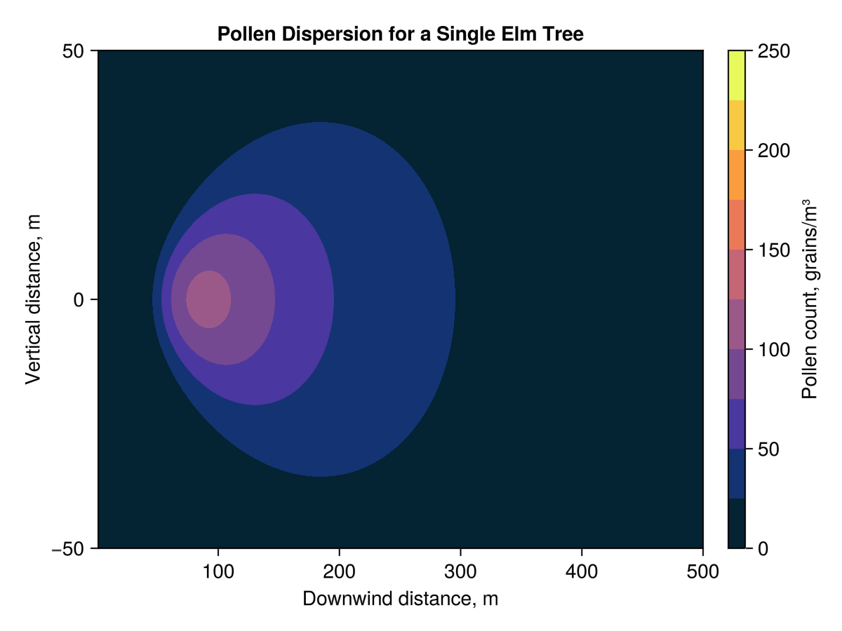
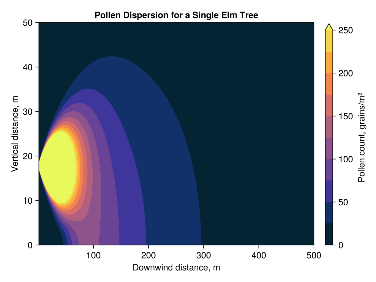
Using this model, the ground level pollen concentration 100 m downwind of the example tree is 105.82 grains m^-3. As shown in the figures below, the pollen is most concentrated in an area from about 75 m to 300 m downwind of the tree. Which is about 2.5 blocks going east-west (city blocks in Edmonton are longer in the north-south direction)
I am left with some questions about how much pollen is actually needed, in the air, for pollination to have a chance. The pollen has to end up on a corresponding flower, so there must be a point where the concentration is just too low to make this likely. Trees do put some effort into improving the odds, they typically flower and disperse pollen before their leaves have meaningfully come back, helping to remove obstructions. The branching structures of trees are both useful for light gathering and provide a large effective area over which their flowers sieve the air for pollen.
On the other side, pollen grains are somewhat fragile too, they can dry out or be damaged by excessive UV exposure. While a single pollen grain may have the potential to make it thousands of meters away from the tree, it may not be viable by the time it gets there.
I would guess, from these calculations, that Elm trees are getting most of their action within 300 m or less. Anything beyond that and the pollen is so dispersed that the odds of it finding a pistil are too low.
A Tree Data Structure
To move from modelling a single tree to an urban forest, I will need a data structure to contain the relevant parameters of a tree. In this case I need both the map location and the location of the tree relative to the origin of the local coordinate system, $x_o, y_o, z_o$. Each tree also has a diameter, height, pollen release rate, and terminal velocity. In this case all the trees are Elm trees, and have the same pollen, but I’m leaving it general in case I want to model something else in the future.
begin

struct Tree{G,L,P,V}
    geopt::G
    xₒ::L
    yₒ::L
    zₒ::L
    DBH::L
    h::L
    P::P
    vₜ::V
end

function Tree(geopt, xₒ, yₒ, DBH; v=vₜ)
    h = crown_height(DBH)
    P = pollen_rate(DBH)
    xₒ, yₒ, zₒ, DBH, h = promote(xₒ, yₒ, zero(yₒ), DBH, h)
    return Tree(geopt, xₒ, yₒ, zₒ, DBH, h, P, v)
end

end;
elm = Tree(nothing, 0u"m",0u"m",DBH)
Tree{Nothing, Quantity{Float64, 𝐋, Unitful.FreeUnits{(m,), 𝐋, nothing}}, Quantity{Float64, 𝐍 𝐓^-1, Unitful.FreeUnits{(grains, s^-1), 𝐍 𝐓^-1, nothing}}, Quantity{Float64, 𝐋 𝐓^-1, Unitful.FreeUnits{(m, s^-1), 𝐋 𝐓^-1, nothing}}}(
    geopt = nothing
    xₒ = 0.0 m
    yₒ = 0.0 m
    zₒ = 0.0 m
    DBH = 0.88 m
    h = 17.803579999999993 m
    P = 317528.8675882605 grains s^-1
    vₜ = 0.032156589905762846 m s^-1
)
I then added a method to ermak that takes a Tree object and returns the concentration of its pollen at a point x, y, and z on the local coordinate system.
function ermak(t::Tree, x, y, z; u=u)
    x′ = x - t.xₒ
    y′ = y - t.yₒ
    z′ = z - t.zₒ
    return ermak(x′, y′, z′; h=t.h, P=t.P, W_set=t.vₜ, W_dep=t.vₜ)
end;
Mapping Elm Pollen in Wîhkwêntôwin
The Ermak equation assumes the local area is a flat Euclidean plane. The earth is not that, and so a central task is going to be defining a local coordinate system that approximates my neighbourhood, Wîhkwêntôwin, as a flat plane. Then I will need to find all of the local trees and place them in this local coordinate system before adding in their individual contributions to the local Elm pollen situation.
Defining the Local Grid
I arbitrarily picked a point more-or-less in the middle of the neighbourhood to act as the origin. My neighbourhood is pretty flat and so I’m going to assume everything is at the same altitude.
using Geodesy
begin

latₒ, lonₒ, altₒ = 53.54100, -113.52141, 671
Δlat, Δlon = 0.015, 0.035

end;
I oriented the grid such that the wind goes from west to east – which is usually the case. Another approach would be to look up the local windrose and orient the grid to the most frequent wind direction with the wind speed as the median wind speed.
I am assuming that the area is locally flat relative to the curvature of the earth. Namely that the distance, in meters, per degree longitude is a constant across the whole neighbourhood – which I calculate from a straight line running through the origin going from the furthest west to the furthest east. Similarly for degrees latitude. This isn’t strictly true but the difference between the distance along the ellipsoid and the locally-flat distance is going to be trivially small, so I can safely ignore it.
begin

Δx = euclidean_distance(LLA(latₒ, lonₒ - Δlon/2, altₒ),
                        LLA(latₒ, lonₒ + Δlon/2, altₒ), wgs84)/Δlon
Δy = euclidean_distance(LLA(latₒ + Δlat/2, lonₒ, altₒ),
                        LLA(latₒ - Δlat/2, lonₒ, altₒ), wgs84)/Δlat
end
function local_coords(lat,lon)
    x = (lon - lonₒ)*Δx
    y = (lat - latₒ)*Δy
    return x, y
end
Why not use Web Mercator?
At first glance it looks like I’m doing a lot of additional work for no reason. I ultimately want to overlay my maps on top of satellite imagery, which will require me to convert everything into Web Mercator. Why not use that as the local coordinate system? Points in Web Mercator are northing and easting in meters on a flat plane.
Unlike UTM, where that kind of thing works out well enough for a lot of situations, there is a lot more distortion with Web Mercator. Especially closer to the poles. I’m not particularly close to the north pole, but more than close enough that the map distortion leads to significant errors when using Web Mercator naively like that.
To demonstrate this I’m going to calculate the distance between my favourite coffee shop, stopgap, and a local park on the other side of the neighbourhood, Oliver park.
begin

stopgap = LLA(53.535618490862944, -113.5118491580413)
oliver_park = LLA(53.54542679826651, -113.52603529325418)

end
dist = euclidean_distance(stopgap, oliver_park, wgs84)
First I calculate the distance along the ellipsoid, which is 1441 m (the same as what Google maps tells me).
Then I convert the coordinates to Web Mercator, which are northing and easting relative to the equator and the prime meridian.
WM = WebMercatorfromLLA(wgs84)
begin

stopgap_wm = WM(stopgap)
oliver_park_wm = WM(oliver_park)

end
wm_dist = √( (stopgap_wm[1] - oliver_park_wm[1])^2
            + (stopgap_wm[2] - oliver_park_wm[2])^2 )
The naive Euclidean distance using Web Mercator is 2423 m, about 68% greater than the true distance. If I set my local grid naively using the northing and easting of Web Mercator, everything would be distorted.
Finding the Neighbourhood Elm Trees
Thankfully, I don’t need to wander the neighbourhood with a GPS unit and a tape measure to find all the local Elm trees and map them. The City of Edmonton has already done that. I filtered the data set to just my neighbourhood and just Ulmus Americana and downloaded it as a csv.
using CSV, DataFrames
trees_df = CSV.read("data/pollen_dispersion/Ulmus_americana_wihkwentowin.csv",
                     DataFrame);
describe(trees_df, :min, :max)
19×3 DataFrame
 Row │ variable                min                                max
     │ Symbol                  Any                                Any
─────┼──────────────────────────────────────────────────────────────────────────────────────────────
   1 │ ID                      155206                             619701
   2 │ NEIGHBOURHOOD_NAME      WÎHKWÊNTÔWIN                       WÎHKWÊNTÔWIN
   3 │ LOCATION_TYPE           Alley                              Park
   4 │ SPECIES_BOTANICAL       Ulmus americana                    Ulmus americana Patmore
   5 │ SPECIES_COMMON          Elm, American                      Elm, American
   6 │ GENUS                   Ulmus                              Ulmus
   7 │ SPECIES                 americana                          americana
   8 │ CULTIVAR                Brandon                            Patmore
   9 │ DIAMETER_BREAST_HEIGHT  5                                  110
  10 │ CONDITION_PERCENT       0                                  65
  11 │ PLANTED_DATE            1990/01/01                         2024/09/25
  12 │ OWNER                   Parks                              Parks
  13 │ Bears Edible Fruit      false                              false
  14 │ Type of Edible Fruit
  15 │ COUNT                   1                                  1
  16 │ LATITUDE                53.5346                            53.5496
  17 │ LONGITUDE               -113.536                           -113.51
  18 │ LOCATION                (53.534594143551985, -113.510361…  (53.549586375568154, -113.530880…
  19 │ Point Location          POINT (-113.50950085882668 53.53…  POINT (-113.53589639202552 53.54…
What I would like is a vector of Trees. I could have added a column to the dataframe with Tree objects when it was created, but I’m not using the dataframe for anything else so I didn’t really see the point.
begin
trees = Vector{Tree}()

for row in eachrow(trees_df)
    lat, lon = row.LATITUDE, row.LONGITUDE
    DBH = row.DIAMETER_BREAST_HEIGHT*1u"cm" |> u"m"
    pt = LLA(lat,lon,altₒ)
    x, y = local_coords(lat, lon).*1u"m"
    tree = Tree(pt,x,y,DBH)
    push!(trees, tree)
end

end
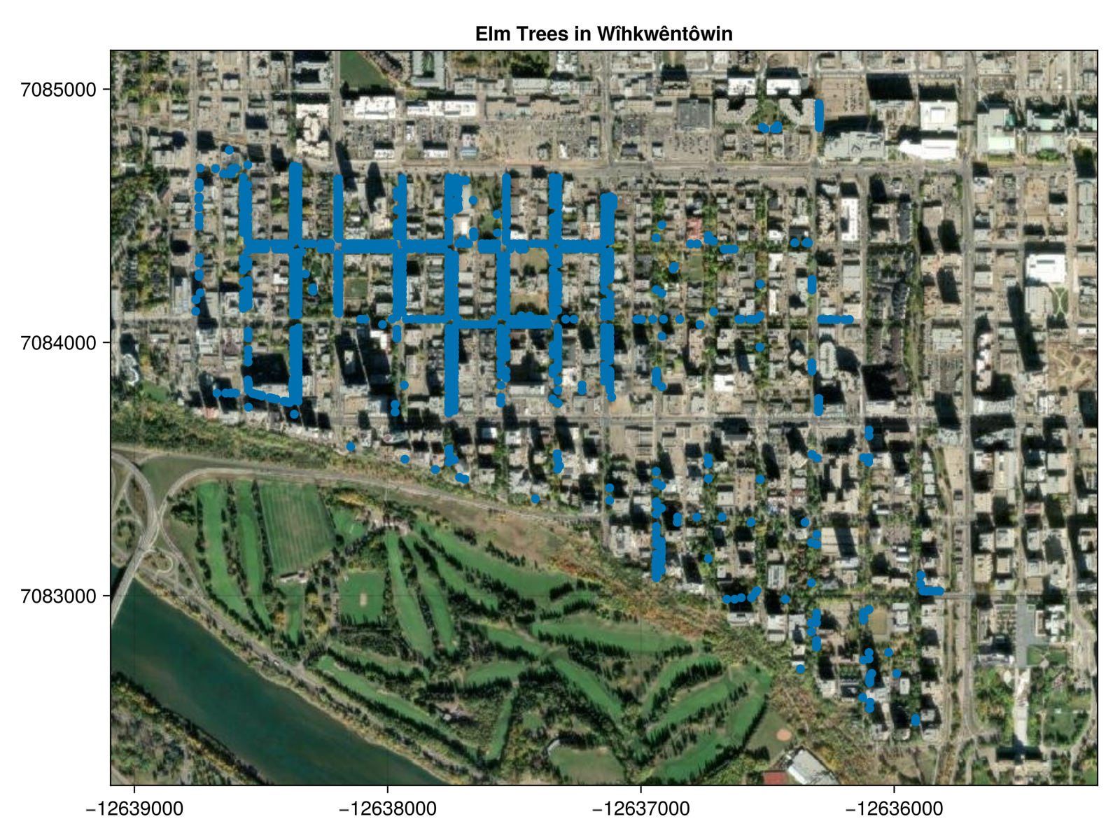
There are 996 Elm trees in Wîhkwêntôwin alone. That’s impressive, we have a pretty great urban forest.
trees[1]
Tree{LLA{Float64}, Quantity{Float64, 𝐋, Unitful.FreeUnits{(m,), 𝐋, nothing}}, Quantity{Float64, 𝐍 𝐓^-1, Unitful.FreeUnits{(grains, s^-1), 𝐍 𝐓^-1, nothing}}, Quantity{Float64, 𝐋 𝐓^-1, Unitful.FreeUnits{(m, s^-1), 𝐋 𝐓^-1, nothing}}}(
    geopt = LLA(lat=53.53695945675063°, lon=-113.51201340003675°, alt=671.0)
    xₒ = 623.0131311454173 m
    yₒ = -449.74535157065054 m
    zₒ = 0.0 m
    DBH = 0.2 m
    h = 9.04518 m
    P = 10810.758180096327 grains s^-1
    vₜ = 0.032156589905762846 m s^-1
)
I am assuming that pollen is additive and doesn’t alter the properties of air at all. The concentration of pollen from multiple trees is just the concentration of pollen from each tree added together.
ermak(trees::Vector{Tree}, x, y, z; u=u) =
    sum( ermak.(trees, x, y, z; u=u) );
Mapping Wîhkwêntôwin
Now that I have a set of trees and a bounding box, I need to generate some actual maps. I am going to use Tyler.jl to download the map tiles and make them plot-able in Makie. For which I need to give it a bounding box for the neighbourhood and identify a map provider. I am using the imagery from ESRI.
using Tyler
wihkwentowin = Rect2f(lonₒ - Δlon/2, latₒ - Δlat/2, Δlon, Δlat);
provider = Tyler.TileProviders.Esri(:WorldImagery);
I have defined a helper function to take a tree and return the appropriate Web Mercator coordinates to map on top of the ESRI imagery.
function map_tree(tree::Tree)
    x, y, _ = WM(tree.geopt)
    return Point2f(x,y)
end
Mapping all of the trees in the data set matches what I expected: they are mostly boulevard trees and the northwest corner of the neighbourhood is much more densely forested with Elm.
Mapping the Pollen from all Elm Trees
Now I have all the tools in place to generate concentration contours for Elm pollen and plot them on top of the ESRI imagery for my neighbourhood. First, I create a helper function to convert grid points in Web Mercator to local grid coordinates, then return the concentration at that point with contributions from all 996 Elm trees.
If I was doing this for the whole city I might want to first filter out all the Elm trees that are too distant from or downwind of the point of interest – since they won’t contribute anything.
LLA_WM = LLAfromWebMercator(wgs84)
function map_ermak(x, y)
    lla = LLA_WM([x,y,altₒ])
    local_x, local_y = local_coords(lla.lat, lla.lon).*1u"m"
    return ustrip(ermak(trees, local_x, local_y, 0u"m"))
end
I then divide the neighbourhood into a grid of 10,000 points and calculate the concentration at each point.
# defining the bounds of the grid

begin

xₗ, yₗ, _ = WM(LLA(latₒ - Δlat/2, lonₒ - Δlon/2, altₒ))
xᵤ, yᵤ, _ = WM(LLA(latₒ + Δlat/2, lonₒ + Δlon/2, altₒ))

end;
begin

xs = range(xₗ, xᵤ; length=100)
ys = range(yₗ, yᵤ; length=100)

zs = map_ermak.(xs, ys')

end;
Finally I overlay a contour plot on top of the ESRI imagery, showing everywhere with a pollen concentration >10 grains m^-3
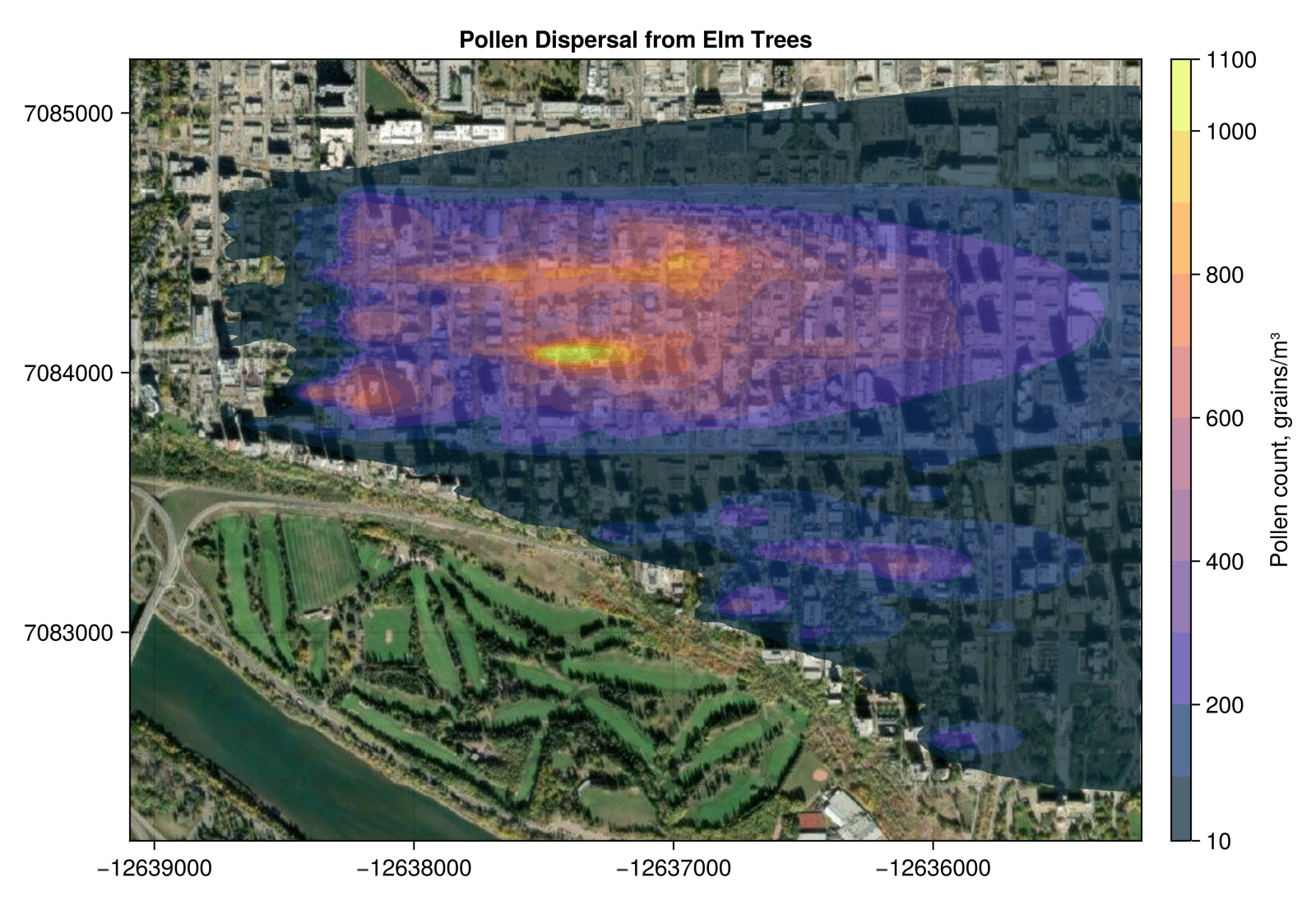
A major limitation to this style of dispersion modelling, especially in a neighbourhood like mine dominated by large apartment buildings, is that building downwash effects are not being accounted for. The Elm trees are at a similar height or shorter than the buildings around them. This model essentially ignores the buildings other than their contribution to surface roughness – reflected in the dispersion parameters $\sigma_y$ and $\sigma_z$. Short of doing a CFD model of the neighbourhood, I don’t think there is an easy way around that. Probably this would work better in neighbourhoods like Highlands or Ritchie which have mature Elm trees but where housing is mostly older homes, less than 2 stories, with yards spacing them out from each other.
A limitation to this specific example is that I haven’t included all the Elm trees in adjacent neighbourhoods – Westmount in particular. This under counts the Elm pollen on the west side of Wîhkwêntôwin. I can imagine one producing maps like this, for the whole city, based on which trees are producing pollen in any given week showing where the peak pollen action is. A where not to park your car map, if you want to avoid washing your windshield every morning, or where to avoid if you are allergic to tree pollen.
For a complete listing of code used to generate data and figures, please see the corresponding pluto notebook
References
- Briggs, Gary A. Diffusion Estimation for Small Emissions. Preliminary Report. Oak Ridge, TN: Air Resources Atmospheric Turbulence and Diffusion Laboratory, NOAA. 1973. doi: 10.2172/5118833
- Brush, Grace S. and Lucien M. Brush Jr. "Transport of Pollen in a Sendiment-Laden Channel: A Laboratory Study." American Journal of Science 272, no. 4 (1972): 359-381
- Ermak, Donald L. "An Analytical Model for Air Pollutant Transport and Deposition from a Point Source." Atmospheric Environment 11 (1977): 231-237 doi: 10.1016/0004-6981(77)90140-8
- Griffiths, R. F. "Errors in the use of the Briggs parameterization for atmospheric dispersion coefficients." Atmospheric Environment 28, no. 17 (1994):2861-2865 doi: 10.1016/1352-2310(94)90086-8
- Katz, Daniel S. W., Jonathan R. Morris, and Stuart A. Batterman. "Pollen Production for 13 Urban North American Tree Species: Allometric Equations for Tree Trunk Diameter and Crown Area." Astrobiologia (Bologna) 36, no. 3 (2020): 401-415 doi: 10.1007/s10453-020-09638-8
- McPherson, E. Gregory, Natalie S. van Doorn, Paula J. Peper. Urban Tree Database and Allometric Equations. Albany, CA: U. S. Department of Agriculture, Forest Service, Pacific Southwest Research Station. 2016. doi: 10.2737/PSW-GTR-253
Comments