\[\begin{align} \eta_t &= 100\;\text{ }(\text{total compression ratio}) \\[10pt] n &= 3\;\text{ }(\text{number of stages}) \\[10pt] \eta &= \eta_t^{\frac{1}{n}} \\[10pt] &= 100^{\frac{1}{3}} \\[10pt] &= 4.64 \end{align}\]
Previously I evaluated hydrogen as a fuel gas from the perspective of an end user – someone who purchases utility natural gas, at pressure, for use in combustion devices like boilers and heaters. From that perspective, hydrogen is not an unreasonable conversion, with material compatibility being the primary concern. In this post I’m going to look at it from the perspective of the gas utility.
From my previous analysis, I showed that the same piping operating at the same pressures delivers approximately the same energy, in terms of higher heating value, in systems in full hydrogen service as those in natural gas service. So, for an end user of natural gas (such as me, it’s how I heat my home) making some modifications to the fired equipment and getting a stream of hydrogen versus natural gas is a plausible pathway to low-carbon heating. That doesn’t entirely hold up for the utility company providing the gas, however, as there is an additional cost associated with compressing hydrogen over natural gas, which might make such systems impractically expensive to operate. At least that is the question I’m looking to answer here: is distributing hydrogen fuel gas to residential or industrial customers through a distribution network like natural gas feasible or not?
The full economic analysis of hydrogen as a fuel gas versus some other low carbon source of energy would so strongly depend on local factors – the local cost of electricity versus hydrogen, whether that region is subject to a carbon tax and how that tax works, etc. – that I don’t think much can be generalized. The economics of hydrogen, where I live, where natural gas is abundant and widely used, export infrastructure is limited, and the carbon tax largely excludes all but the largest industrial emitters, is pretty different from a place where all natural gas is imported at large expense, or with a very different approach to carbon pricing.
Instead of pursuing a complete technoeconomic analysis of hydrogen, a pretty ambitious topic for a short blog post, I am going to focus on the single factor that is often bandied about online to justify the conclusion that hydrogen distribution is infeasible: the work needed to compress the gas in the pipeline system. I want to show where that number comes from and think about what it might tell us about the system overall.
The Situation
We already know that natural gas distribution systems are feasible, there is one delivering natural gas to my house right now and it is also delivering natural gas to the chemical plant I work at, the gas fired power plant that is powering my laptop right now, etc. To some extent we also already know that hydrogen distribution systems are feasible as they already exist, the longest hydrogen transmission pipeline in Europe is >1000km long and there are >700km of hydrogen pipelines in the United States.1 However those are primarily for supplying hydrogen as a feedstock to chemical and petrochemical facilities, not quite the same use case as hydrogen as a fuel gas.
A reasonable approach to considering the feasibility of a hypothetical hydrogen transmission system is to compare it to an equivalent natural gas system. This is basically what I’ve already done for pipe-flow when looking at hydrogen blending: once the hydrogen is in the pipe and at pressure, everything works from that point down. What remains to be seen is whether it is feasible to get it into the pipe and at pressure. Specifically how much more work does it take to compress hydrogen to line pressure than natural gas?
The standard equation for determining the work, \(\dot{w}_{g}\), to compress a mass flowrate \(\dot{m}\) of gas from a pressure of \(p_1\) to \(p_2\) is234
4 Strictly speaking this is an approximation as it neglects the change in kinetic energy of the fluid, but for small compression ratios, less than ~5, it is appropriate
\[ \dot{w}_{g} = \dot{m} \int_{p_1}^{p_2} v dp \]
This is related to the isentropic work through the isentropic efficiency, \(\varepsilon_{i}\)
\[ \varepsilon_{i} \dot{w}_{g} = \dot{m} \int_{p_1}^{p_2} v dp \vert_{isentropic} \]
Where the integral of the specific volume \(v\) is taken along an isentropic path. Real compressors are not isentropic, but compressor manufacturers provide tables or figures giving the isentropic efficiency, with values of 70% - 80% being fairly typical.
I am going to assume that whatever efficiency can be achieved for a standard natural gas compressor can also be achieved with a hydrogen compressor. They may be different compressors, but the isentropic efficiency is something of a design choice. The ratio of work for a hydrogen system to a natural gas system, \(r\), is then
\[ r = { {\dot{w}_{g}}_{H2} \over {\dot{w}_{g}}_{NG} } = { \left( \varepsilon_{i} \dot{w}_{g} \right)_{H2} \over \left( \varepsilon_{i} \dot{w}_{g} \right)_{NG} } = { \left( \dot{m} \int_{p_1}^{p_2} v dp \right)_{H2} \over \left( \dot{m} \int_{p_1}^{p_2} v dp \right)_{NG} } \]
The integrals, though, do not have to be tackled directly, recalling the differential for (specific) enthalpy
\[ dh = v dp + T ds \]
Integrating from state 1 to state 2 along an isentropic path (i.e. \(ds = 0\)) gives:
\[ \int_{h_1}^{h_2} dh = h_2 - h_1 = \int_{p_1}^{p_2} v dp \]
Thus the ratio we’re looking for is given by:
\[ r = { \dot{m}_{H2} \over \dot{m}_{NG} } { {\Delta h}_{H2} \over {\Delta h}_{NG} } \]
It is important to note that state 2 is not the same for hydrogen and natural gas. Since the integration is along an isentropic path, state 2 is at a pressure of \(p_2\) and a temperature \(T_2\) defined by \(s_1 = s_2\) and the entropy of hydrogen and natural gas are, in principle, different.
Compressors typically don’t raise pressures all the way from, say, atmospheric pressure to the 200-1500psi working pressures of natural gas transmission lines in a single stage. For one, as gases are compressed they heat up and that large temperature rise can damage a compressor. Usually compression is accomplished with a series of stages with interstage cooling. This work ratio is really only valid for a single stage.
Suppose we are evaluating a system that uses a multi-stage compressor to take gas at ambient conditions, in this case suppose 1bar and 15C, to a relatively high transmission line pressure of 100bar using 3 stages, Figure 1. The overall compression ratio is 100, with 3 stages this gives a per stage ratio of
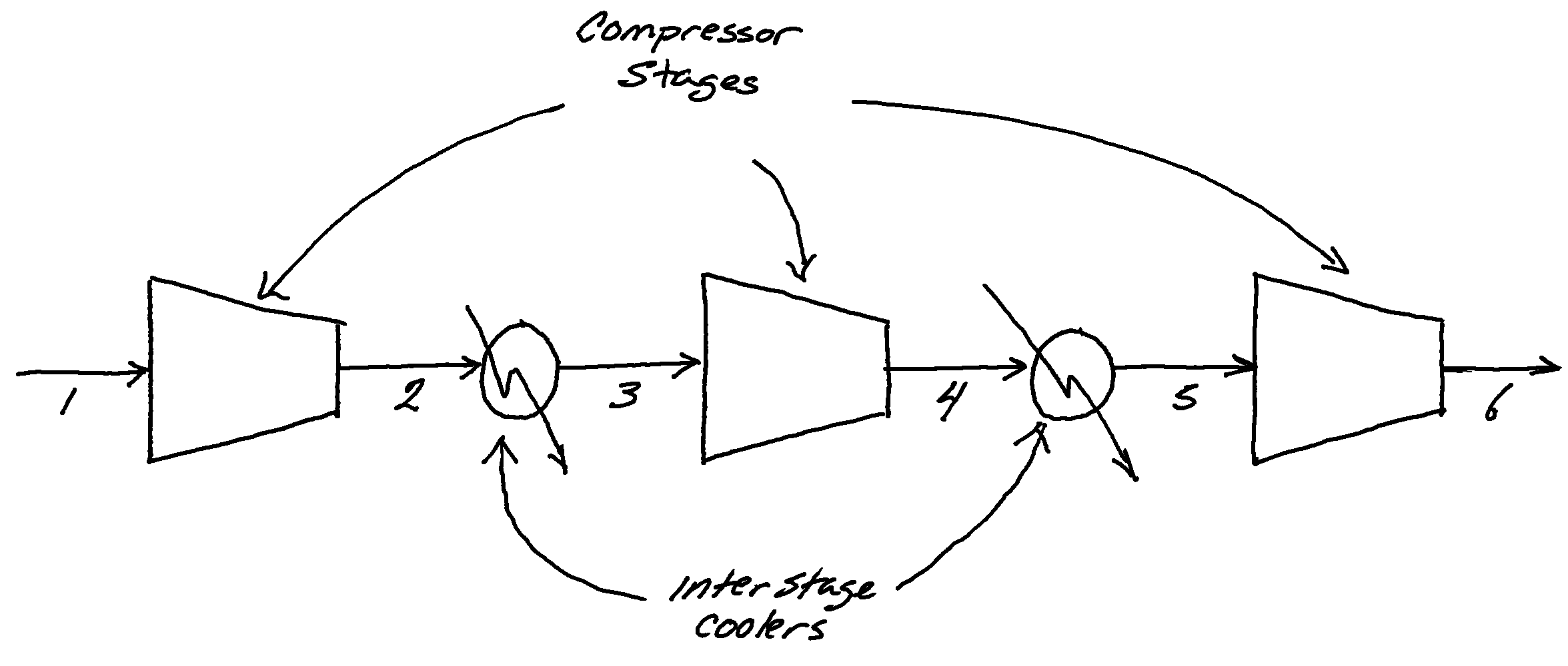
Suppose, for simplicity, the interstage coolers bring the gas temperature down to 15C:
- the first stage compresses the gas from 1 bar to 4.6 bar
- the second stage compresses the gas from 4.6 bar to 21.5 bar
- the last stage compresses the gas from 21.5 bar to 100.0 bar
With the inlet gas to each stage being at 15C and exiting at some temperature which is determined from the energy balance and isentropic efficiency.
The total work required to compress the gas is then
\[ r_{T} = { \dot{m}_{H2} \over \dot{m}_{NG} } { \left( {\Delta h}_{1 \to 2} + {\Delta h}_{3 \to 4} + {\Delta h}_{5 \to 6} \right)_{H2} \over \left( {\Delta h}_{1 \to 2} + {\Delta h}_{3 \to 4} + {\Delta h}_{5 \to 6} \right)_{NG} } \]
The Ideal Gas Case
A useful first approach to most problems in life5 is to assume an ideal gas. It allows one to build some intuition about the problem and how fluid non-ideality may change the results. Starting with an ideal gas in stream 1 being isentropically compressed to stream 2,6 and equating the specific enthalpies
5 for chemical engineers at least
\[ s_0 + \int_{T_0}^{T_1} {c_p \over T} dT - R \log { p_1 \over p_0 } = s_0 + \int_{T_0}^{T_2} {c_p \over T} dT - R \log { p_2 \over p_0 } \]
Assuming \(c_p\) is a constant this simplifies to
\[ c_p \log{ T_2 \over T_1 } = R \log{p_2 \over p_1} \]
For an ideal gas \(c_p - c_v = R\), giving
\[ \log{T_2 \over T_1} = { {c_p - c_v} \over c_p} \log{ p_2 \over p_1} \]
\[ {T_2 \over T_1} = \left( p_2 \over p_1 \right)^{1 - \frac{1}{k}} \]
A well known result. The enthalpy of an ideal gas with constant \(c_p\) is just \(c_p T\), so we have:
\[ \Delta h = c_p \Delta T = c_p \left( T_2 - T_1 \right) \]
\[ = c_p T_1 \left( {T_2 \over T_1} -1 \right) \]
\[ = c_p T_1 \left( \left( p_2 \over p_1 \right)^{1 - \frac{1}{k}} - 1 \right) \]
From the ideal gas law, \(T = \frac{pv}{R}\)
\[ \Delta h = \frac{c_p}{R} p_1 v_1 \left( \left( p_2 \over p_1 \right)^{1 - \frac{1}{k}} - 1 \right) \]
\[ = {k \over {k-1}} p_1 v_1 \left( \left( p_2 \over p_1 \right)^{\frac{k-1}{k}} - 1 \right) \]
Which allows us to write the work ratio, for a single stage, compressing an ideal gas with constant heat capacity, as:
\[ r = { \dot{m}_{H2} \over \dot{m}_{NG} } { {v_1}_{H2} \over {v_1}_{NG} } {C_{NG} \over C_{H2}} { { \eta^{C_{H2}} -1 } \over { \eta^{C_{NG}} - 1} } \]
where \(C = \frac{k-1}{k}\). From the ideal gas law the ratio of specific volumes is just the ratio of molar weights \[ { {v_1}_{H2} \over {v_1}_{NG} } = { MW_{NG} \over MW_{H2} } \]
\[ r = { \dot{m}_{H2} \over \dot{m}_{NG} } { MW_{H2} \over MW_{NG} } {C_{NG} \over C_{H2}} { { \eta^{C_{H2}} -1 } \over { \eta^{C_{NG}} - 1} } \]
and, since the inlet streams are all at the same temperature
\[ r_T = r \]
Furthermore, if we assume \(k_{NG} \approx k_{H2}\) then
\[ r = { \dot{m}_{H2} \over \dot{m}_{NG} } { MW_{NG} \over MW_{H2} } \]
This is where I’ve encountered what I consider a serious error: assuming an equal mass flowrate of the two fuels. Making this assumption gives
\[ r = { MW_{NG} \over MW_{H2} } \]
using Unitful, Clapeyronideal_hydrogen = ReidIdeal(["hydrogen"])
ideal_natural_gas = ReidIdeal(["methane"])\[\begin{align} MW_{NG} &= 16.04\,\mathrm{kg}\,\mathrm{kmol}^{-1} \\[10pt] MW_{H2} &= 2.02\,\mathrm{kg}\,\mathrm{kmol}^{-1} \\[10pt] r &= \frac{MW_{NG}}{MW_{H2}} \\[10pt] &= \frac{16.04\,\mathrm{kg}\,\mathrm{kmol}^{-1}}{2.02\,\mathrm{kg}\,\mathrm{kmol}^{-1}} \\[10pt] &= 7.94 \end{align}\]
This gives a work ratio of 7.9, leading us to conclude that it will take 7.9× the power to run a hydrogen transmission system than a similar natural gas system.
I think this is a mistake because the goal is not to deliver the same mass flowrate but the same thermal energy (combustion energy). Supposing we are seeking to deliver the same energy in terms of higher heating value
\[ hv_{H2} \dot{m}_{H2} = hv_{NG} \dot{m}_{NG} \]
\[ { \dot{m}_{H2} \over \dot{m}_{NG} } = { hv_{NG} \over hv_{H2} } \]
and so
\[ r = { hv_{NG} \over hv_{H2} } { MW_{NG} \over MW_{H2} } \]
where \(hv\) is the specific higher heating value (or gross heating value)
\[\begin{align} hv_{NG} &= 55.58\,\mathrm{MJ}\,\mathrm{kg}^{-1}\;\text{ }(\text{GPSA Handbook}) \\[10pt] hv_{H2} &= 141.95\,\mathrm{MJ}\,\mathrm{kg}^{-1}\;\text{ }(\text{GPSA Handbook}) \\[10pt] r &= \frac{hv_{NG}}{hv_{H2}} \cdot \frac{MW_{NG}}{MW_{H2}} \\[10pt] &= \frac{55.58\,\mathrm{MJ}\,\mathrm{kg}^{-1}}{141.95\,\mathrm{MJ}\,\mathrm{kg}^{-1}} \cdot \frac{16.04\,\mathrm{kg}\,\mathrm{kmol}^{-1}}{2.02\,\mathrm{kg}\,\mathrm{kmol}^{-1}} \\[10pt] &= 3.11 \end{align}\]
This gives a work ratio of 3.1, quite a bit smaller of an estimate.
But the assumption that \(k_{H2} \approx k_{NG}\) is perhaps not a good one, so we should explore how compression effects differ even as ideal gases.
k(gas) = isobaric_heat_capacity(gas, 1u"bar", 288.15u"K") /
         isochoric_heat_capacity(gas, 1u"bar", 288.15u"K")
\[\begin{align} k_{H2} &= 1.41\;\text{ }(\text{Clapeyron.jl, at 1bar and 15C}) \\[10pt] C_{H2} &= 1 - \frac{1}{k_{H2}} \\[10pt] &= 1 - \frac{1}{1.41} \\[10pt] &= 0.29 \\[10pt] k_{NG} &= 1.31\;\text{ }(\text{Clapeyron.jl, at 1bar and 15C}) \\[10pt] C_{NG} &= 1 - \frac{1}{k_{NG}} \\[10pt] &= 1 - \frac{1}{1.31} \\[10pt] &= 0.23 \\[10pt] r_{ig} &= \frac{hv_{NG}}{hv_{H2}} \cdot \frac{MW_{NG}}{MW_{H2}} \cdot \frac{C_{NG} \cdot \left( \eta^{C_{H2}} - 1 \right)}{C_{H2} \cdot \left( \eta^{C_{NG}} - 1 \right)} \\[10pt] &= \frac{55.58\,\mathrm{MJ}\,\mathrm{kg}^{-1}}{141.95\,\mathrm{MJ}\,\mathrm{kg}^{-1}} \cdot \frac{16.04\,\mathrm{kg}\,\mathrm{kmol}^{-1}}{2.02\,\mathrm{kg}\,\mathrm{kmol}^{-1}} \cdot \frac{0.23 \cdot \left( 4.64^{0.29} - 1 \right)}{0.29 \cdot \left( 4.64^{0.23} - 1 \right)} \\[10pt] &= 3.25 \end{align}\]
This gives a work ratio of 3.25, which shows that our original approximation was reasonable: accounting for differences in isentropic expansion factor, \(k\), changes our estimate by only 5.0%.
The Real Gas Case
To account for non-ideality we need to lose some generality. The ideal gas case ultimately doesn’t depend on what the initial and final conditions are (since all of that cancels out) but for real gases how non-ideal they are depends strongly on the actual pressures and temperatures of the system.
I am going to use a volume translated Peng Robinson cubic equation of state for both hydrogen and methane.
real_hydrogen = PR(["hydrogen"];
                   idealmodel=ReidIdeal,
                   alpha=TwuAlpha,
                   translation=PenelouxTranslation)
real_natural_gas = PR(["methane"];
idealmodel=ReidIdeal,
alpha=TwuAlpha,
translation=PenelouxTranslation)Clapeyron.jl does not define functions for finding the enthalpy as a function of pressure and entropy, so we will need to first find the isentropic temperature, and then calculate the enthalpy.
using Roots: find_zero

function isentropic_temperature(gas, p1, T1, p2)
    s1 = entropy(gas, p1, T1)
    k_ig = k(gas)
    T2_guess = T1*(p2/p1)^(1-1/k_ig)
    T2 = find_zero( T -> entropy(gas, p2, T) - s1, T2_guess)
    return T2
end
First, the molar enthalpy difference for hydrogen
\[\begin{align} p_{1} &= 1\,\mathrm{bar} \\[10pt] T_{1} &= 288.15\,\mathrm{K} \\[10pt] p_{2} &= 4.64\,\mathrm{bar} \\[10pt] T_{2H2} &= 447.3\,\mathrm{K}\;\text{ }(\text{Clapeyron.jl}) \\[10pt] H_{1H2} &= -283.16\,\mathrm{J}\,\mathrm{mol}^{-1}\;\text{ }(\text{Clapeyron.jl}) \\[10pt] H_{2H2} &= 4344.03\,\mathrm{J}\,\mathrm{mol}^{-1}\;\text{ }(\text{Clapeyron.jl}) \\[10pt] {\Delta}H_{H2} &= H_{2H2} - H_{1H2} \\[10pt] &= 4344.03\,\mathrm{J}\,\mathrm{mol}^{-1} + 283.16\,\mathrm{J}\,\mathrm{mol}^{-1} \\[10pt] &= 4627.18\,\mathrm{kJ}\,\mathrm{kmol}^{-1} \end{align}\]
Then the molar enthalpy difference for natural gas
\[\begin{align} T_{2NG} &= 404.45\,\mathrm{K}\;\text{ }(\text{Clapeyron.jl}) \\[10pt] H_{1NG} &= -369.79\,\mathrm{J}\,\mathrm{mol}^{-1}\;\text{ }(\text{Clapeyron.jl}) \\[10pt] H_{2NG} &= 4015.67\,\mathrm{J}\,\mathrm{mol}^{-1}\;\text{ }(\text{Clapeyron.jl}) \\[10pt] {\Delta}H_{NG} &= H_{2NG} - H_{1NG} \\[10pt] &= 4015.67\,\mathrm{J}\,\mathrm{mol}^{-1} + 369.79\,\mathrm{J}\,\mathrm{mol}^{-1} \\[10pt] &= 4385.45\,\mathrm{kJ}\,\mathrm{kmol}^{-1} \end{align}\]
Finally, the work ratio of compressing hydrogen versus natural gas: \[ r_{rg} = { \dot{m}_{H2} \over \dot{m}_{NG} } { {\Delta h}_{H2} \over {\Delta h}_{NG} } = \frac{hv_{NG}}{hv_{h2}} \frac{MW_{NG}}{MW_{H2}} { {\Delta H}_{H2} \over {\Delta H}_{NG} } \]
\[\begin{align} r_{rg} &= \frac{hv_{NG}}{hv_{H2}} \cdot \frac{MW_{NG}}{MW_{H2}} \cdot \frac{{\Delta}H_{H2}}{{\Delta}H_{NG}} \\[10pt] &= \frac{55.58\,\mathrm{MJ}\,\mathrm{kg}^{-1}}{141.95\,\mathrm{MJ}\,\mathrm{kg}^{-1}} \cdot \frac{16.04\,\mathrm{kg}\,\mathrm{kmol}^{-1}}{2.02\,\mathrm{kg}\,\mathrm{kmol}^{-1}} \cdot \frac{4627.18\,\mathrm{kJ}\,\mathrm{kmol}^{-1}}{4385.45\,\mathrm{kJ}\,\mathrm{kmol}^{-1}} \\[10pt] &= 3.28 \end{align}\]
In this case the ideal gas law estimate and the estimate using a cubic equation of state differ by only 1.0%.

The difference does become more pronounced at higher pressures, see Figure 2, but even at stage three the work ratio for the real gases differs from the ideal gas case by only 6.0%.
In online discussions I have seen it claimed that the difference in work – why so much more energy is required to compress hydrogen over natural gas – is due to some obscure feature of hydrogen’s phase diagram. I would say that is false. The main reason why hydrogen requires more energy to compress is simply due to its low molecular weight. That hydrogen has a high energy density, on a mass basis, offsets this greatly when hydrogen and natural gas are compared on an equivalent energy basis, though.
There are additional effects that make hydrogen even more difficult to compress than you would expect, from a pure ideal gas analysis, but they are pretty small unless the working pressures are either huge or the compression ratio is tremendous. Neither of which are particularly relevant for a gas transmission system using normal compressors and typical pipeline pressures.
Final Thoughts
I wrote this post to address some misconceptions that I’ve encountered regarding hydrogen7 and in particular the rhetorical device of finding one single fact about hydrogen and taking that to mean some project or another has been “debunked”. Real engineering projects are just too complex for that to be a useful exercise. Reality always depends on a great many factors.
7 is this all just an extended response to a thread on mastodon? I mean… sort of
When considering my gas bill, at home, the dominant factor for the cost of natural gas is the cost to procure it in the first place (i.e. source it from wells, process it in gas plants). Transmission costs are relatively low (granted I live in a province where it just comes out of the ground, so the transmission distances are pretty low too). I imagine this would be the same for a hydrogen fuel gas system as well: the dominant cost will be the making of hydrogen.
Is the fact that a hydrogen fuel distribution system would require >3× the energy to operate mean that such a system is impractical? That really depends. It could be that a large, continent spanning, transmission system for hydrogen such as natural gas distribution employs in North America is rendered totally infeasible by the increased transmission costs. But then again, why should hydrogen be so geographically constrained? Natural gas is constrained by geology but presumably one could make green hydrogen wherever there is water and renewable power. Perhaps blue hydrogen is best built on top of the existing natural gas infrastructure: send natural gas across the continent and convert it to hydrogen closer to the end use.
I think it is clear, considering the problem more broadly, that hydrogen is unlikely to be a simple drop in replacement with the current infrastructure: infrastructure optimized for natural gas is not infrastructure optimized for hydrogen. But there are real opportunities for repurposing some parts of the natural gas infrastructure for hydrogen that shouldn’t be ignored.
I think the dreams of existing gas fired power plants simply retrofitting to hydrogen and continuing on as before are looking increasingly like a relic from a bygone era. But this has less to do with the practicalities of delivering hydrogen and much more to do with the price of renewables and storage, which continue to plumet. But for other industries, with other heating demands, perhaps there is a compelling case to be made.
I say all of this as someone who is broadly skeptical of the hype around hydrogen. I think it is being pursued mostly as a saviour of fossil fuels and not as a technology that actually best solves the problems which face us as we transition to a low carbon future. But there are also a lot of really smart engineers working on projects centered around low-carbon hydrogen, and I imagine they know what they are doing.
References
Boyce, Meherwan P., Victor H. Edwards, Terry W. Cowley, Hugh D. Kaiser, Wayne B. Geyer, David Nadel, Larry Skoda, Shawn Testone, and Kenneth L. Walter. “Transport and Storage of Fluids.” In Perry’s Chemical Engineers’ Handbook, edited by Don W. Green, 8th ed. New York: McGraw Hill, 2008.
Gmehling, Jürgen, Bärbel Kolbe, Michael Kleiber, and Jürgen Rary. Chemical Thermodynamics for Process Simulation. Weinheim, DE: Wiley-VCH Verlag & Co., 2012.
GPSA. Engineering Data Book. 13th ed. Tulsa, OK: Gas Processors Suppliers Association, 2012.
Sendehboudi, Sohrab, and Bahram Gharbani. Hydrogen Production, Transportation, Storage, and Utilization. Amsterdam: Elsevier, 2025.